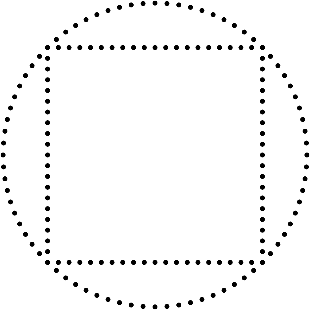
 ver the last few years I’ve often drawn squares using 4 lines made out of dots, and recently I decided it was time to find a more elegant solution. I wanted a simple parametric equation that would draw the whole square in one fell swoop. I searched online and found many different solutions, none of which fit all my criteria. I first considered this equation, which I’ll call solution A. It’s a polar equation for a regular n-gon. So if n=4, we expectedly obtain a square.
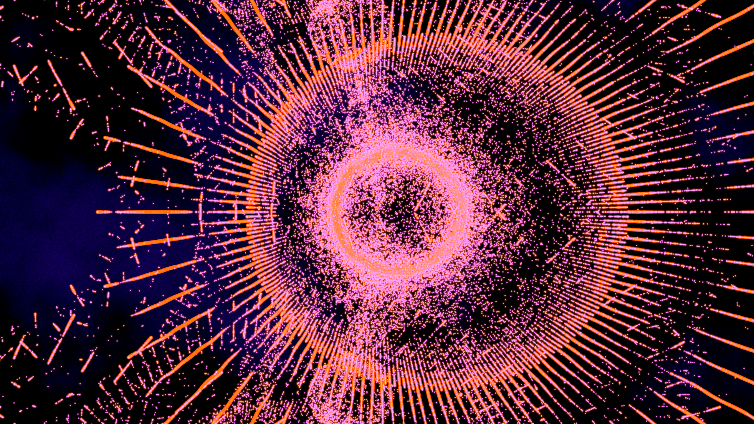
Here is a video that you can download in high resolution format, for free. The video is also on YouTube for those who can’t download the big file.
If you enjoy this work, I invite you to subscribe to my Patreon. You’ll be helping me to create and share more work. There is currently another exclusive high resolution video that patrons can download, and more videos on the way.
Context
I’ve been making a lot of animations like this one, simply for my own enjoyment, and sharing them on social media always feels unsatisfying because of the poor quality of recompressed files. The point of such animations is to lose oneself into all their tiny details, and this is lost on Twitter or Instagram. Even on YouTube and Vimeo, the quality isn’t on par with the original file. I wouldn’t want to watch my own work on a streaming platform, and inviting other people to do so doesn’t feel ideal.
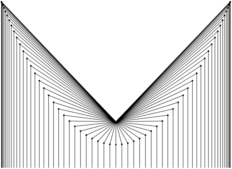 aking connections between mathematical and artistic ideas is a major source of joy for me, and consequently I’m always on the lookout for interesting experiments that I can conduct to get more familiar with different areas of mathematics in ways that feel free and creative. A few weeks ago, I watched a YouTube video by physics and mathematics educator Toby Hendy in which she explains how to draw a parabola using a metaphor inspired by Bob Ross, the late host of The Joy of Painting.
In Hendy’s metaphor, we paint a landscape that contains a horizon, a mountain, and a mushroom situated near the top of the mountain.
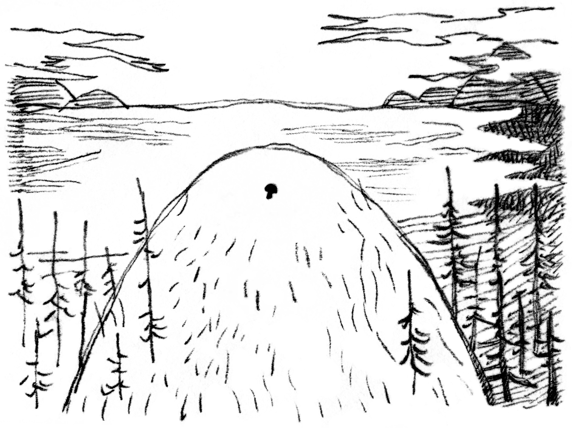
Hendy explains that it’s possible for us to define the contour of the mountain while only knowing the position of the mushroom and the horizon. She proceeds to draw a set of lines projected downward from the horizon, and another set of lines projected from the mushroom at various angles. A parabola then appears at the points where those two sets of lines meet.
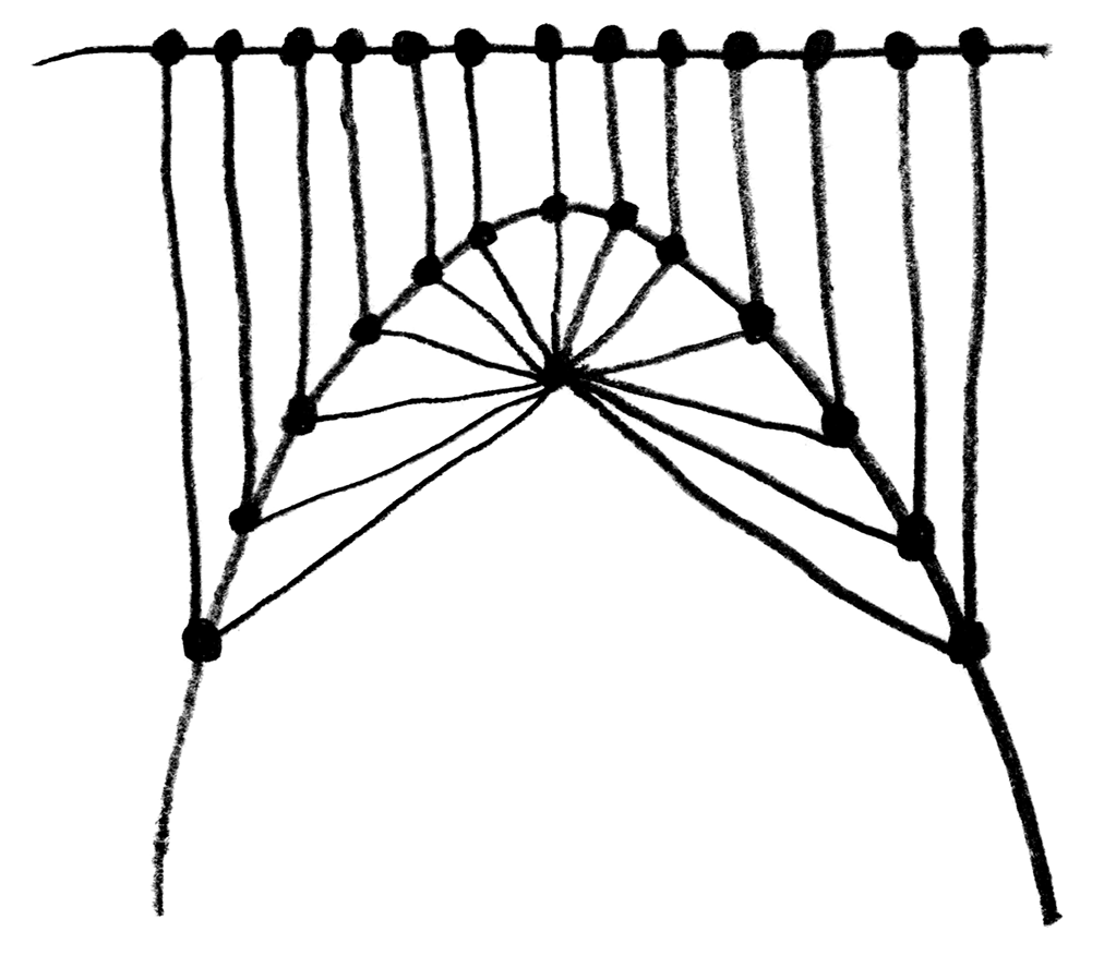
When I saw the parabola appear, I couldn’t quite understand what was happening exactly, so I decided to recreate this experiment in code using p5.js. Here is what I obtained: You can find the code for this animation in the p5.js web editor here.
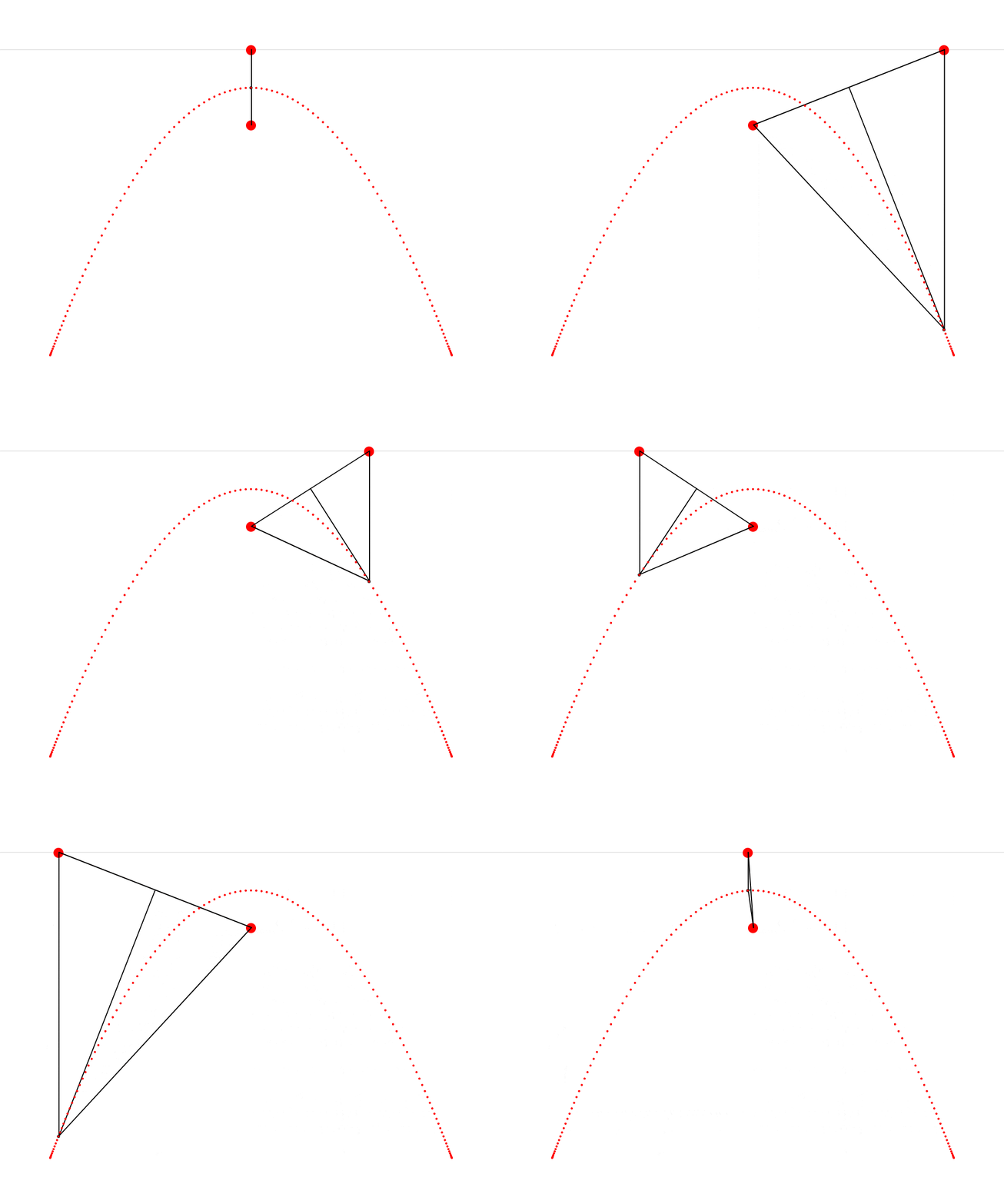
In this animation, we see that it’s possible to construct an isosceles triangle whose first vertex is situated on the horizon, whose second vertex is situated on the mushroom, This point that Hendy makes us imagine as a mushroom is called the focus of the parabola. Wikipedia describes a parabola as “the locus of points in [the] plane that are equidistant from both the directrix and the focus.” The directrix is the horizon in our metaphor. We can thus see that the present exercise makes us replicate this definition very precisely. and whose third vertex traces a parabola. I also cut the isosceles triangle into two right triangles—I feel like this cut clarifies the symmetry that is present in the isosceles triangle and which is so important here.
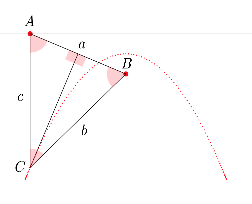
To build this ABC triangle, we must first project a vertical line c downward from the vertex A and another line a between the vertices A and B. We must then calculate the angle A and project a line b from the vertex B to form an angle equal to A (so that ABC is isosceles). Edges b and c of the triangle must then meet at vertex C. When this process is repeated starting from several different points on the horizon, the vertex C of each triangle always falls on the path of the parabola.
Onward to the realm of sounds
One of the first things that came to my mind after I drew a single parabola was that I could now create endless copies of it and turn them into a signal, a parabolic wave.

I got really curious about how this would sound. I first imagined that it would sound something halfway between a sine wave and a triangle wave, because it visually seems to have characteristics of both: a smooth curve and a sharp corner. The parabolic wave also looks very similar to the absolute value of a sine wave, but it is a little bit different, as shown here. This intuition turned out to be wrong.
Below you can listen to a sound file containing three notes: an A at 220 Hz played with a sine wave, then a parabolic wave, and then a triangle wave. You’ll hear that the parabolic wave in the middle doesn’t sound at all like it is halfway between the sine wave and the triangle wave.

Last winter, I started to work on an acoustic piano multi-sampler for SuperCollider. The earliest versions had many issues, and my budding programming skills in sclang did not allow me to fix them. But I’ve used the instrument a lot since then, and I’ve improved the code along the way. I plan to keep working on the instrument as I keep using it, but I’m thinking that it could already be useful for other people if they are interested. So here it is.
The instrument uses a public domain sample pack I used this same sample pack for the soundtrack of my short film Étude for Cellular Automata no 2, although in this case I used a single piano sample and shifted its pitch down over several octaves to generate every note. It creates a very warbly sound that was appropriate for the intended atmosphere. I also used the piano samples in this live coding experiment.that you can download from freesound.org. You’ll need to create an account to download it, but it’s free to join, and free to download, and I highly recommend this website.
Below is the entirety of the code for the sampler, along with some Pbind examples to try it out. It is free software distributed under an Apache 2.0 licence. You can also find this code on GitHub.
// Run this block of code once the server is booted.
// You also need to make sure that the packLocation variable
// is set to the actual location of the downloaded sample pack.

(
var pianoSamples, pianoFolder, makeLookUp, indices, pitches, dynAmnt, maxDyn, maxNote,
packLocation = "/21055__samulis__vsco-2-ce-keys-upright-piano/",
quiet = false;

dynAmnt = if (quiet, {2}, {3});
maxDyn = if (quiet, {1}, {2});
maxNote = if (quiet, {46}, {1e2});
pianoSamples = Array.new;
pianoFolder = PathName.new(packLocation);
pianoFolder.entries.do({
    |path, i|
    if (i < maxNote, {
        pianoSamples = pianoSamples.add(Buffer.read(s, path.fullPath));
    });
});

makeLookUp = {
    |note, dynamic|
    var octave = floor(note / 12) - 2;
    var degree = note % 12;
    var sampledNote = [1,  1,  1,  1,  2,  2,  2,  3,  3,  3,  3,  3];
    var noteDeltas = [-1, 0,  1,  2, -1,  0,  1, -2, -1,  0,  1,  2];
    var dynamicOffset = dynamic * 23;
    var sampleToGet = octave * 3 + sampledNote[degree] + dynamicOffset;
    var pitch = noteDeltas[degree];
    [sampleToGet, pitch];
};
indices = dynAmnt.collect({|j| (20..110).collect({|i| makeLookUp.(i, j)[0]})}).flat;
pitches = dynAmnt.collect({|j| (20..110).collect({|i| makeLookUp.(i, j)[1]})}).flat;

Event.addEventType(\pianoEvent, {
    var index;
    if (~num.isNil, {~num = 60}, {~num = min(max(20, ~num), 110)});
    if (~dyn.isNil, {~dyn = 0}, {~dyn = floor(min(max(0, ~dyn), maxDyn))});
    index = floor(~num) - 20 + (~dyn * 91);
    ~buf = pianoSamples[indices[index]];
    ~rate = (pitches[index] + frac(~num)).midiratio;
    ~instrument = \pianoSynth;
    ~type = \note;
    currentEnvironment.play;
});

SynthDef(\pianoSynth, {
    arg buf = pianoSamples[0], rate = 1, spos = 0, pan = 0, amp = 1, out = 0, atk = 0, sus = 0, rel = 8;
    var sig, env;
    env = EnvGen.kr(Env.new([0, 1, 1, 0], [atk, sus, rel]), doneAction: 2);
    sig = PlayBuf.ar(2, buf, rate * BufRateScale.ir(buf), startPos: spos, doneAction: 2);
    sig = sig * amp * 18 * env;
    sig = Balance2.ar(sig[0], sig[1], pan, 1);
    Out.ar(out, sig);
}).add;
)

// Below are examples of patterns that show how to use the instrument.
// I recommend running both patterns at the same time,
// they are made to complement each other.

(
var key = 62;
var notes = key + ([0, 3, 7, 10] ++ [-5, 2, 3, 9]);
~pianoRiff.stop;
~pianoRiff = Pbind(
    \type, \pianoEvent,
    \dur, Pseq(0.5!1 ++ (0.25!3), inf),
    \num, Pseq(notes, inf),
    \dyn, Pseq([1, 0, 0, 1], inf),
    \amp, Pseq([0.5, 2, 2, 0.5], inf),
    \pan, Pwhite(-0.75, 0.75, inf),
    \rel, 4
).play(quant: [2]);
)

(
var key = 62 + 36;
var notes = key + [2, -5, 0, -2];
~pianoRiff2.stop;
~pianoRiff2 = Pbind(
    \type, \pianoEvent,
    \dur, Pseq([0.25, 1.75], inf),
    \num, Pseq(notes, inf),
    \dyn, Pseq([1, 1, 1, 1], inf),
    \amp, Pseq([0.5, 1, 1, 0.5], inf),
    \pan, Pwhite(-0.75, 0.75, inf),
    \rel, 4
).play(quant: [2]);
)

(
~pianoRiff.stop;
~pianoRiff2.stop;
)
How to use the sampler
Using the instrument will probably be very straightforward for most users of SuperCollider, but I thought that writing down some instructions could still be useful, particularly for beginners. It’s also an opportunity to talk about the design decisions that went into creating the instrument, and the ways in which it could potentially be improved.
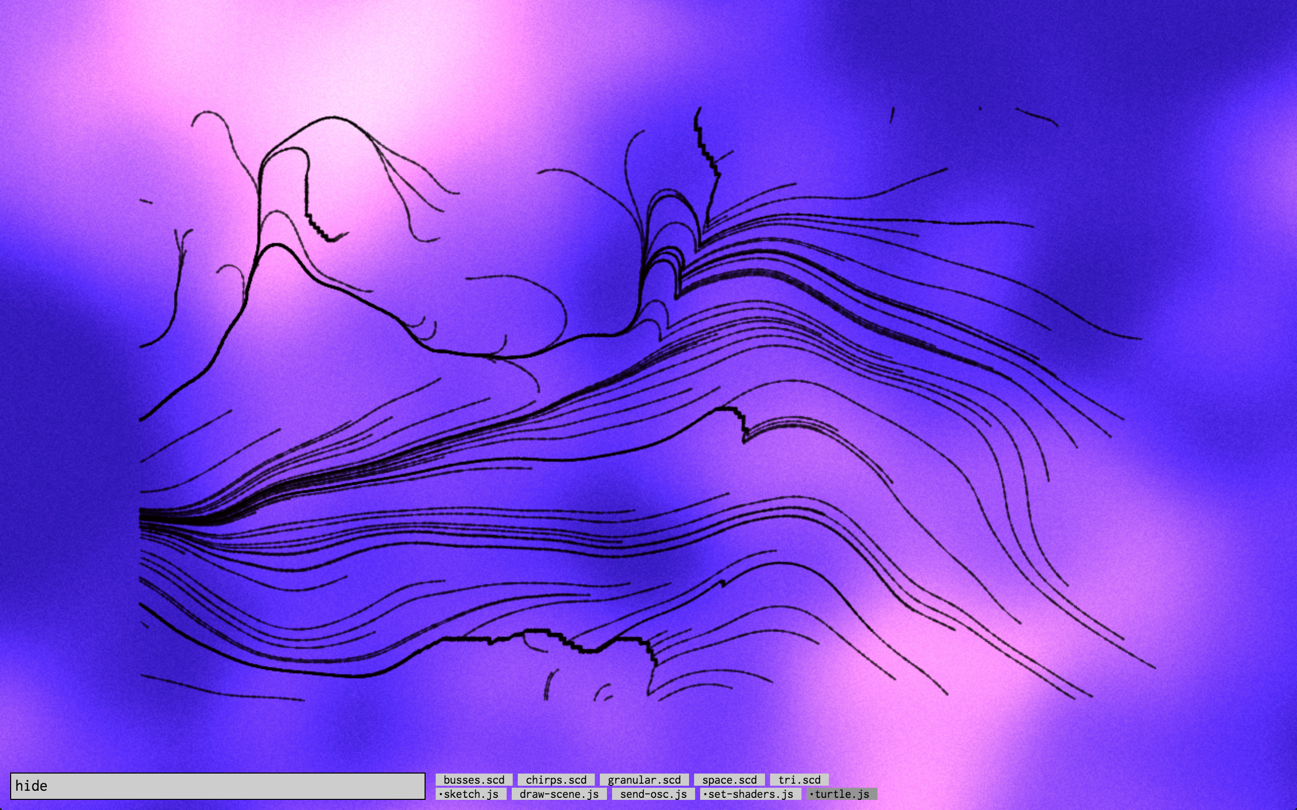
I currently have the vague idea of reusing some concepts from my short film Ravines for a live coding set that I could perform in various ways (as opposed to the short film itself, which exists in a static, definite form). The laptop I use for live coding is quite slow, so I have to really simplify and optimize the original algorithms to be able to run them in real time. It’s an interesting challenge to work around those limitations. The animations in Ravines were too resource-intensive to be rendered in real time. It took around 12 hours to render the whole thing.
As you can see in the still images above and below, my goal is also to play with colour. I enjoy the stark black and white look of Ravines, but I generally prefer to work with colours and I envision my live coding sets as being very warm and colourful. The colourful backgrounds here were created by adapting the fog effect taken from this ShaderToy post.
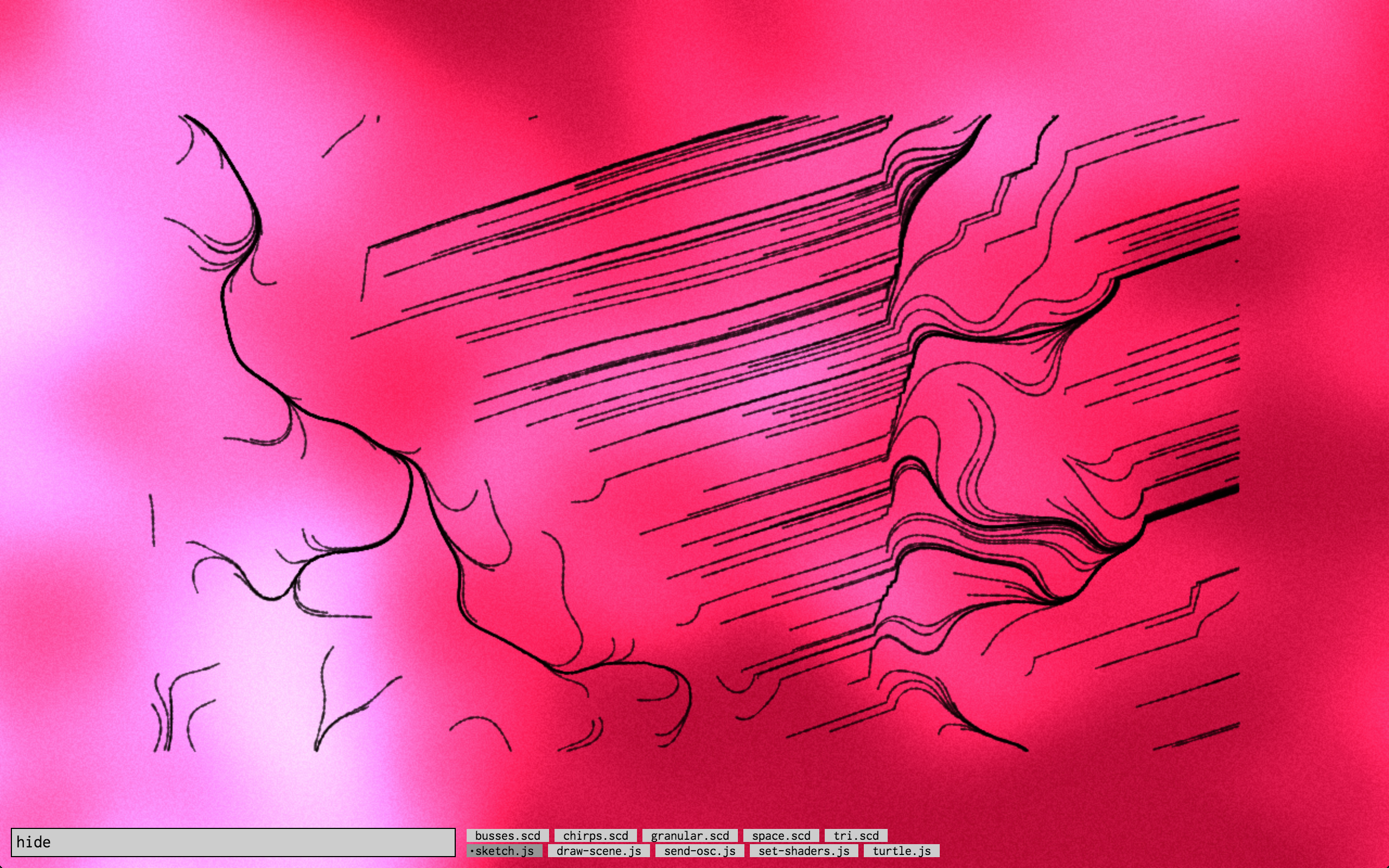
I’m currently learning the basics of wavetable synthesis with SuperCollider, and I will gather my notes and my first musical sketches below. I started to learn with this excellent video by Eli Fieldsteel, who takes part of his material in the documentation of the Shaper class.
It all begins with the creation of a wavetable:
~sig = Signal.newClear(513);
(
~sig.waveFill({
    arg x, y, i;
    // i.linlin(0, 512, -1, 1);
    // sin(x);
    sin(x.cubed * 20);
}, 0, 1);
~sig.plot;
~w = ~sig.asWavetableNoWrap;
~b = Buffer.loadCollection(s, ~w);
)
We create an instance of Signal, we fill it with the waveFill method, we transform it into an instance of Wavetable, and then load it into a Buffer. The expression sin(x.cubed * 20) used to fill the Signal was written arbitrarily and I really love the sound that it produces.
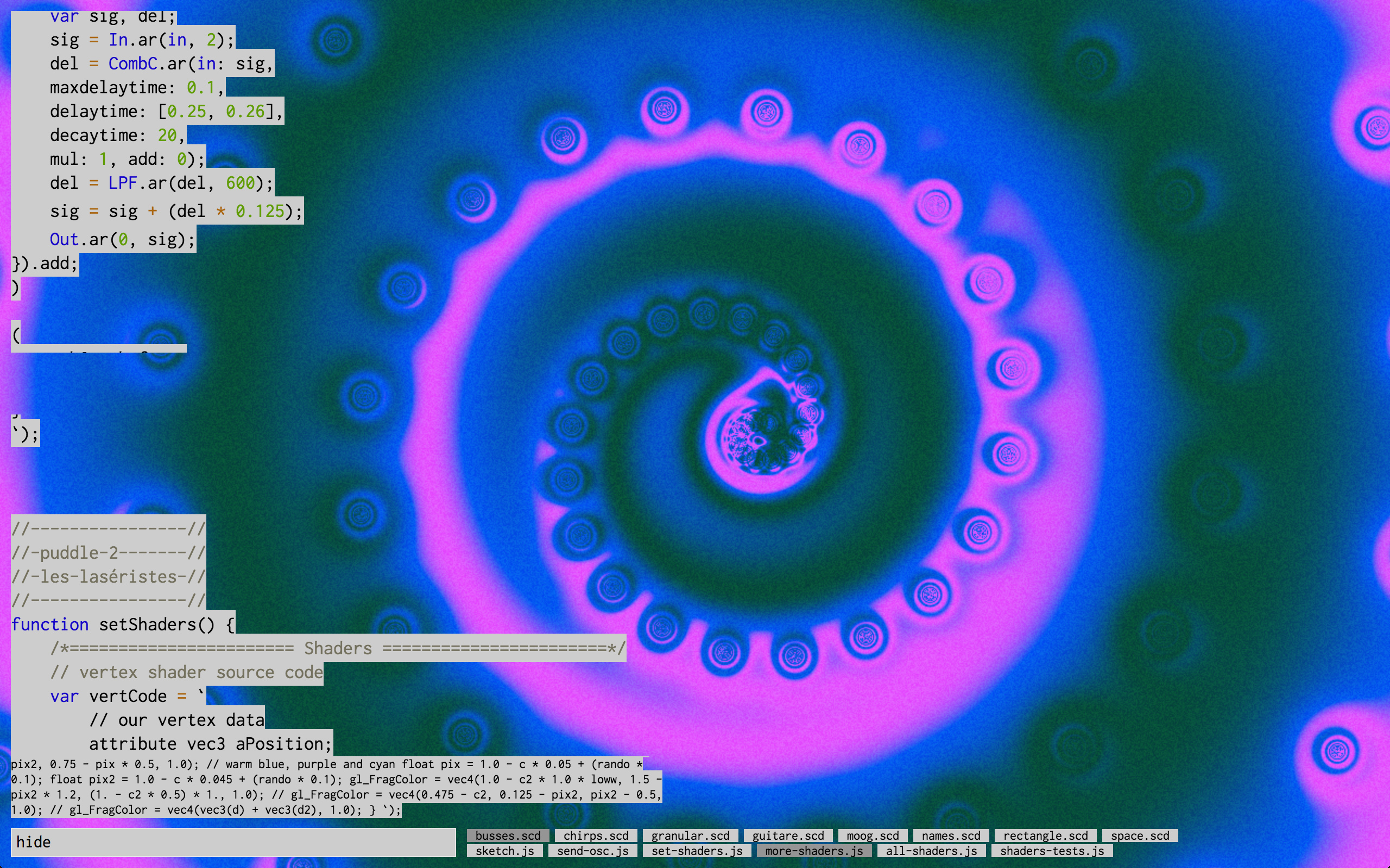
I’m continuing to learn live coding with SuperCollider and WebGL shaders, and I composed another audiovisual set, trying more complicated things that I wasn’t able to do for the first one. I performed this new piece at the concert venue La Vitrola on March 29th 2019, as part of the third edition of Signes vitaux, a series of concerts organised by Rodrigo Velasco (Yecto) and Toplap Montréal.
Unfortunately, my computer is not fast enough to render this piece to disk while I perform it, so for now I’m unable to share a completed version of this work.
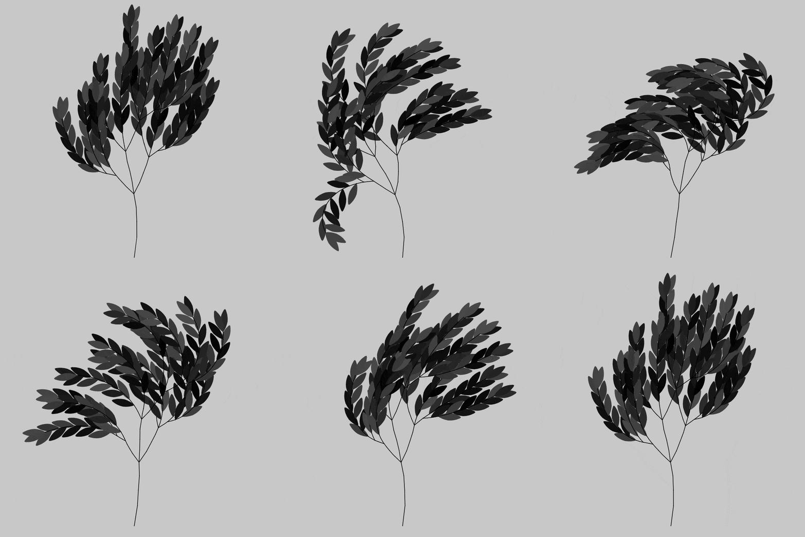
The code written to make the animation above and the one below can be found on the noise-loops branch of the Evolutionary Botany GitHub repository. The OpenSimplex noise implementation that I’m using is called SimplexNoiseJS and was written by Mark Spronck.
While getting to know the basics of machine learning, I stumbled on some notions of calculus, something that I’m very unfamiliar with but that I would love to understand. I have been thinking for a while about devising some small experiments that would allow me to familiarize myself with mathematical concepts in an intuitive way. So this sudden need to understand a bit of calculus seemed like a good opportunity to delve into this.
The animation below is one of those experiments. It helped me to familiarize myself with the notions of limits and tangents. A line is tangent to a circle when its slope is identical to the slope of the circle at the point where they meet. This slope is calculated by taking two different points on the circle, and by then diminishing almost infinitely the distance between those two points. This is what I have done while writing the code for this animation. I was interested in what kinds of shapes I would obtain by playing with these notions, and I ended up with a dense mesh of tangent lines evenly distributed around a circle. I then got curious about how the mesh would “react” if I morphed the shape of the circle, and this animation was the result.
