What the Walls Feel

In the fall of 2019, Toronto composer Frank Horvat published an album of minimalist chamber music The album is titled What Goes Around and you can stream it on his website. Do check it out, it is wonderful music. and decided to hire filmmakers to transform each album track into a short experimental video. This ongoing project now features the work of fellow Montreal animators Moïa Jobin-Paré and Sunny Stanila, Toronto artist Matthew Maaskant, and me.

You can watch my video on Frank’s YouTube channel. It is made entirely using free, open source, and custom-made software, and all the code written to create the video is also distributed as free software. You can find the code here.

Visualizing musical minimalism

The album track I found most inspiring for my video was a melancholy piece for six clarinets titled What the Walls Feel as they Stare at Rob Ford Sitting in his Office. In his programme notes for the piece, Frank explains the inspiration behind this peculiar title. It’s in the style of musical minimalism, so it’s built on the slow transformation of repeated patterns—introducing new variations within carefully restricted bounds. Like most minimalist pieces, it also doesn’t feature a lot of dynamics (contrasts between quiet and loud parts), and instead immerses the listener in a rich sequence of microscopic changes.

I’m a lover of musical minimalism, having listened to some of its luminaries like Steve Reich, Meredith Monk, and Julius Eastman, for countless hours, so the task of responding to this music with images was an exciting one. It was also clear that geometric and algorithmic animation was the perfect tool to visually recreate the idea of tiny variations within restricted bounds. Minimalist music is strongly connected to process music, which Steve Reich defines as “pieces of music that are, literally, processes”. In the domain of algorithmic art, everything is a process—algorithms are simply sets of instructions that define processes. Algorithmic art is thus often refered to as procedural art, and the software Processing is one of the most important tool in the field.

The cover art for some important minimalist albums like Steve Reich’s Music for 18 Musicians and Drumming, and Jon Gibson’s Two Solo Pieces, which all feature dense geometric patterns, also exemplify this connection.

Searching for a visual system

It’s my second time doing commission animation work using algorithmic art. The first time was for a music video directed by Pascaline Lefebvre, an illustrator, author, and filmmaker from Montréal. Most of the animation in the video was hand-drawn by Pascaline, and I contributed by animating the flocks of birds that you can see during a few moments in the video. The flocking algorithms that I used for this video were inspired by Daniel Shiffman’s videos on the subject. All the code I wrote for this project can be found here.

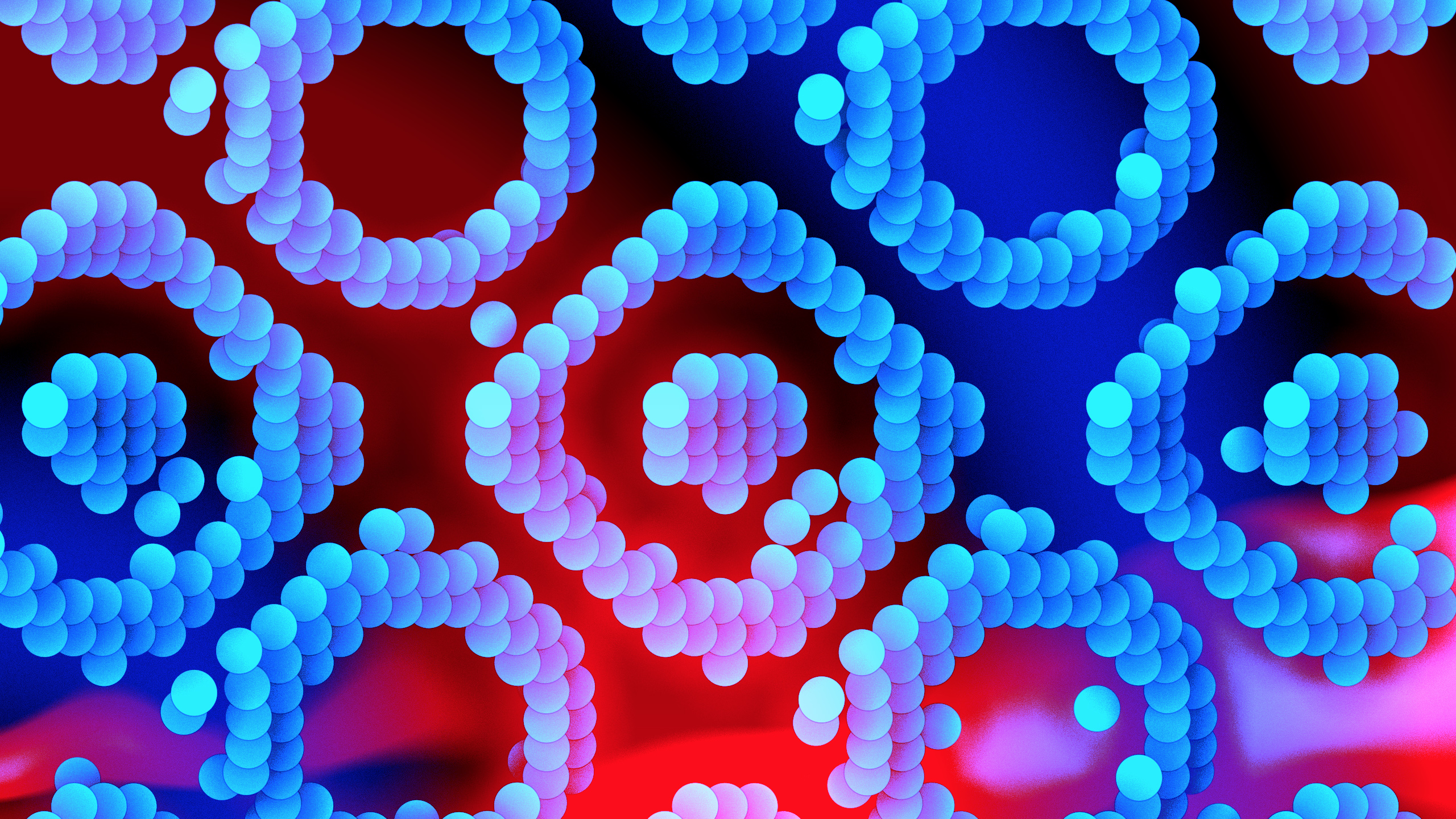
This time around, I listened to Frank’s music a lot while sketching an assortment of ideas. I eventually had an idea that I found very fitting for the music: a wall of small dots moving in different choreographies, forming into a series of intricate patterns.

I sketched out a prototype using the p5.js web editor. Here it is: You can also see this sketch right next to its code in the p5.js web editor. It will let you easily modify any elements of the sketch and see the results immediately.

The wall was a good visual anchor for the whole thing considering the title of the musical piece. Even if the dots are moving in smooth oscillations, it’s very clear that they are ultimately laid out in a strict grid. I enjoy the tension between those two phenomena, and thought it was a good visual metaphor for the music. The walls are ruminating, contorting themselves into worried thoughts.

Building the software

The film was made entirely by writing custom-made software. The film is itself a program—when this program runs, it either plays the film or renders it to disk. It is distributed as free, open source software, and you can find all the code for it here. You are free to run it, modify it, and distribute modified versions. My work was also greatly inspired by the software p5.js, created by Lauren McCarthy and her team.

To write the film, I used another software that I’m currently writing, called Les environs (French for The Surroundings). Les environs is also distributed as free software and you can download it here. Les environs is a live coding environment—it allows to write and modify a program while it is running. It was first designed for the live performance of animation and music. I used it in a few group concerts in Montréal in 2019. Adapting this performative tool for the needs of a film production was a really interesting challenge. I ended up building various modules for all steps of the production: animation, editing, coloration, compositing, rendering.

Below is what the software looks like when I work on the video.

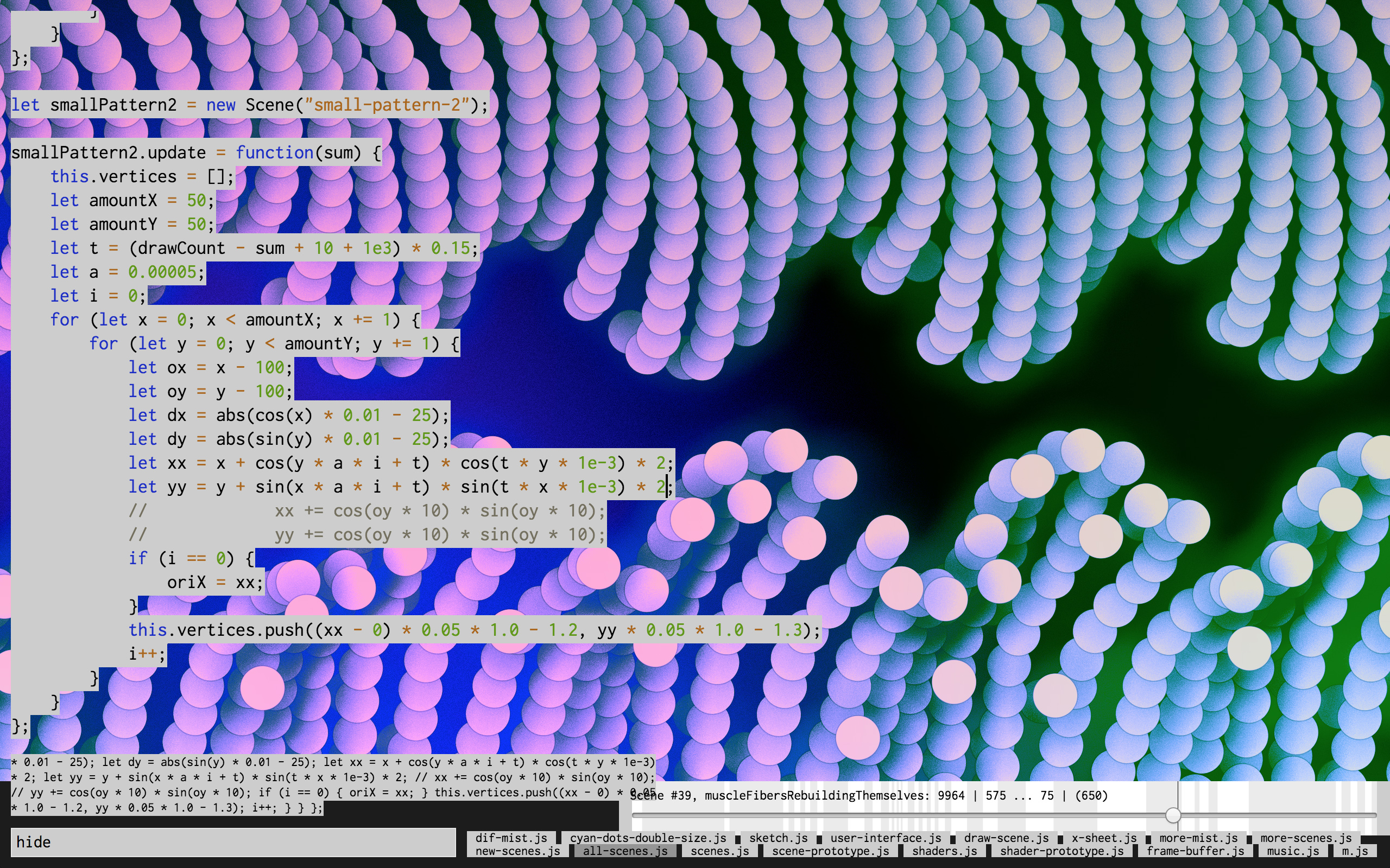
The frame of the film covers most the screen, and a portion of the code is superimposed over it (the code can easily be hidden to reveal the entire image). Near the bottom right of the screen sits the timeline, where all scenes appear as a succession of white and light grey bars. Along the bottom edge are the tabs, which determine what portion of the code is currently displayed. The code can be modified while the film is running, and it affects the film immediately. For example, while the timeline is visually represented, it can only be modified with the code, and changing the length of a scene in the code will automatically update the visual timeline. It’s also possible to zoom into smaller sections of the timeline, still using text commands.

Coloration research

One of my favourite enhancement that I made to my system for this project was the possibility of blending multiple image layers using various blending functions—the typical blending functions found in Photoshop and After Effects (multiply, add, soft light, etc.). More precisely, my system doesn’t rely on linear stacks of layers like Photoshop or After Effects. It can instead be non-linear graphs of layers, or networks of layers. Story time: my first experience putting an animation film together was made with the antique software USAnimation by Toon Boom. In this 2001 awn article, a screenshot of USAnimation’s “Camera module” shows how it relied on this powerful idea of graphs of layers. After transitioning to After Effects a long time ago, I always felt limited by the restrictive system of linear stacks of layers. It is quite a joy to finally go back to graphs. I found a replica of these blending functions on a very helpful blog post from 2009, and because this code is distributed as free, open source software, it was possible for me to integrate it to my system. My layer system currently doesn’t exist in a visual form, so putting several layers together is done strictly via coding, and you have to imagine the layer order in your mind.

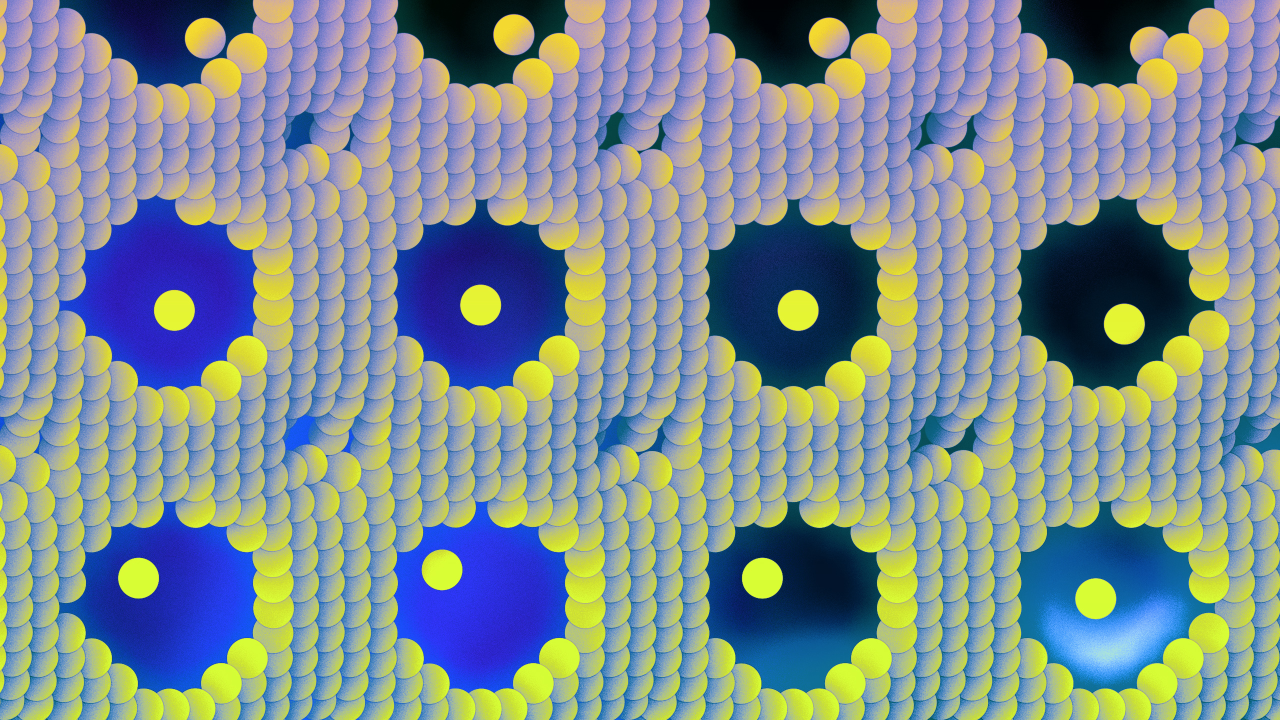
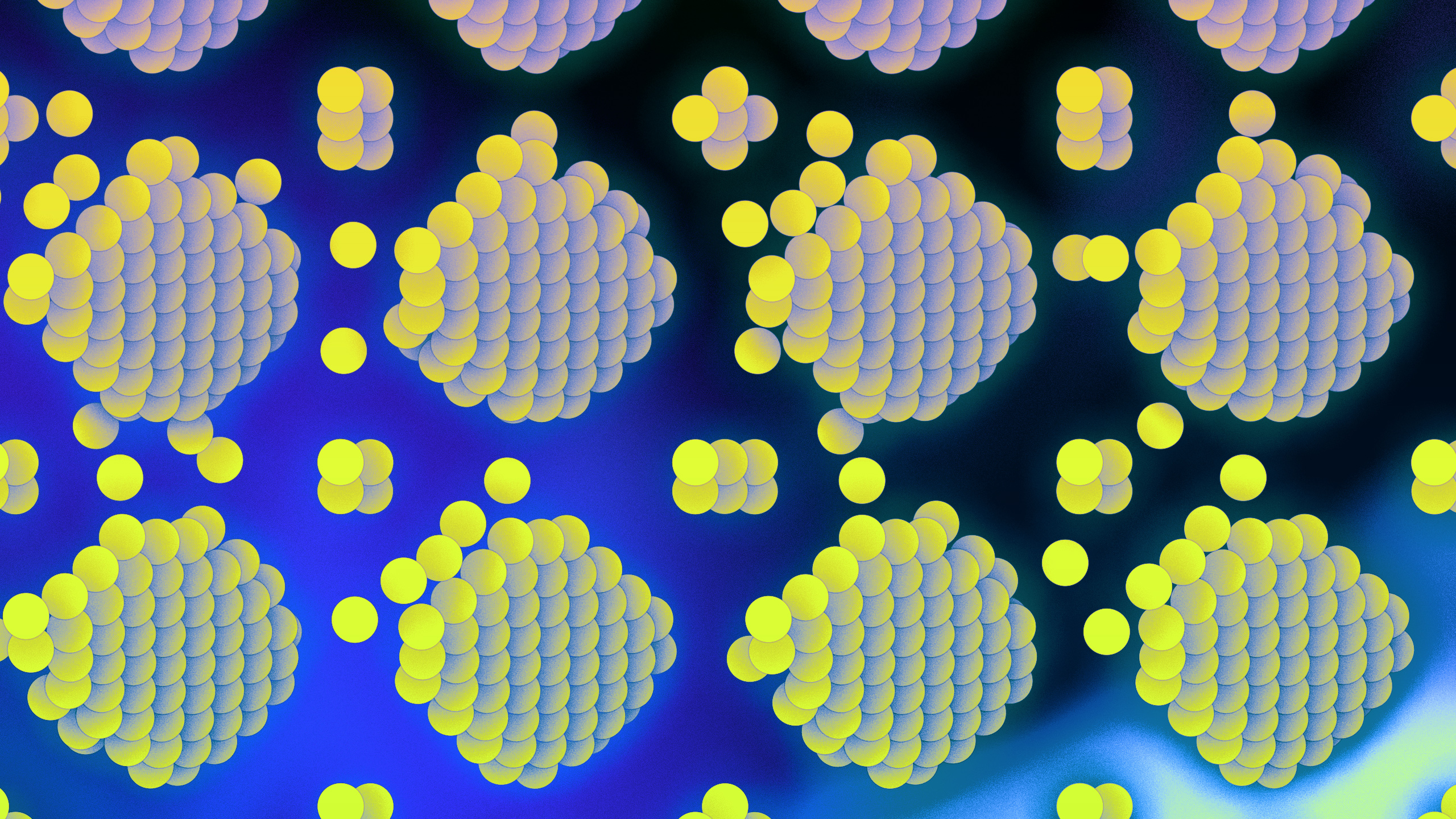
This improved system of layers was very useful during the coloration research, which ended up being quite extensive. Below are some examples of this research. My research tended to lead me towards bright and joyous colours because I enjoy them a lot, but they did not fit the tone of the piece of music at all. The music needed a quieter, somber, sadder palette.

I also experimented a lot with colour transitions from scene to scene, but that did not work either. The musical colour of Frank’s piece is so steady and finds so much of its force and its character in this unchanging, unrelenting stubbornness, that introducing a new colour palette at any point in the film felt completely unearned—it felt like the image simply drifted away from the music, exactly the opposite of what I wanted. It also felt like I was simply trying to cram more pretty colours in the film, which is indeed what was happening.

The mathematics behind the film

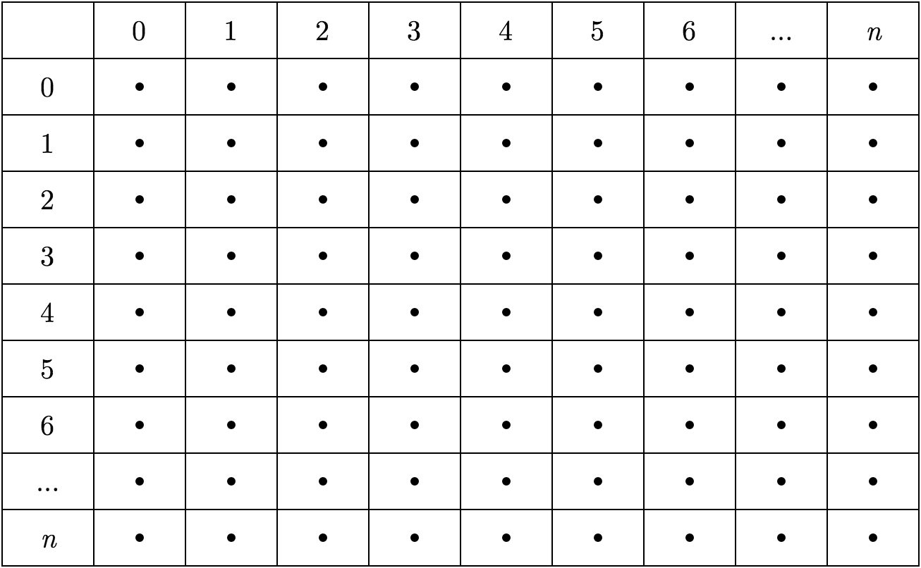
The system on which the whole film is built is a two-dimensional grid of dots, with an $x$ horizontal axis and a $y$ vertical axis. Each dot occupies one cell within the grid. For example, the dot at the top left has a position of $x=0,y=0$.

Each dot in this grid is able to move in space. Its initial position in space is defined by the $x$ and $y$ values of the cell in which it is contained. But then, the dot’s final position $p$ is calculated by applying a mathematical transformation, which is usually a parametric equation. As an example, here is the transformation that was applied on the animation seen above in this article.

An identical copy of this equation is sent to all the dots, but because each dot has a different $x$ and $y$ value within the grid, the result of the equation is different for each dot. So this equation has three inputs: $x$, $y$, and $t$. The $x$ and $y$ values are the position of the dot within the two-dimensional grid. The third value, $t$, is the moment in time. It is a value that starts at $0$ when the animation begins and it is simply incremented on each frame of animation. In this case, it is incremented by $\pi /60$, an arbitrary number that I chose after trying different numbers and figuring how at which speed the animation was the most interesting to watch. I find it interesting to point out the amount of arbitrary decisions that are taken in the design of such systems, because I remember when I was starting out a few years ago, looking at other people’s code, I was often under the impression that all parameters of any given system were chosen for some mystical reasons that were out of my grasp, while really, most of this is trying out a ton of different values and slowly approaching what looks the nicest to you. In this case, $\pi /60$ also means that this function will start repeating itself every $120$ frames, since the sine and cosine functions repeat themselves over $2\pi$. The $t$ value is identical for each dot—time goes forward at the same speed for all dots.

So once this formula is calculated for each dot, the $p_x$ and $p_y$ values of each dot will determine its exact position in space. Note that any dot can fly outside of its origin cell—the cell’s purpose is to give its dot an initial position, not to constrain the dots’ movements within bounds.

Endless variations

What I enjoyed about this system when I started to play with it is the implied infinity of variations that it can produce. By changing any parameters from the formula, but more importantly by writing entirely different formulas, I could get an infinite amount of different choreographies of dots.

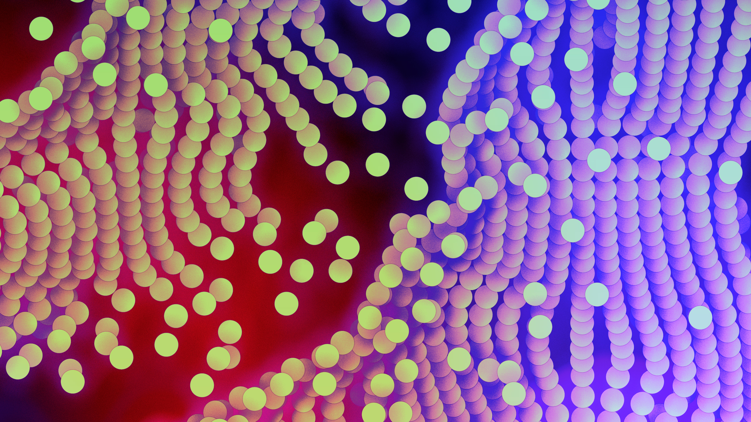
For example, the equation below gave me a very big surprise. The resulting animation doesn’t look like a pattern of oscillation anymore. It looks like it was generated by a complicated algorithm that moves data around.

This is the equation used in the opening scene of the video, where the dots all move in straight lines, resembling cars stuck in traffic.

Closing thoughts

Responding to Frank’s music with my animations was an inspiring project to undertake. And getting the opportunity to work more on building my animation software was quite a gift: I ended up with results that I could not have expected when the project started. There are millions of ways in which my current system could be improved. I hope to get the opportunity to keep this work going.